Tutorial v2.0.0¶

The aim of this tutorial is to give a basic introduction to the main workflow of scousepy. Each stage will be described below along with some of the important customisable keywords. All data for the tutorial can be found here, along with some example scripts.

Data¶

This tutorial utilises observations of N2H+ (1-0) towards the Infrared Dark Cloud G035.39-00.33. This data set was first published in Henshaw et al. 2013.. These observations were carried out with the IRAM 30m Telescope. IRAM is supported by INSU/CNRS (France), MPG (Germany) and IGN (Spain). The data file is in fits format and is called

n2h+10_37.fits

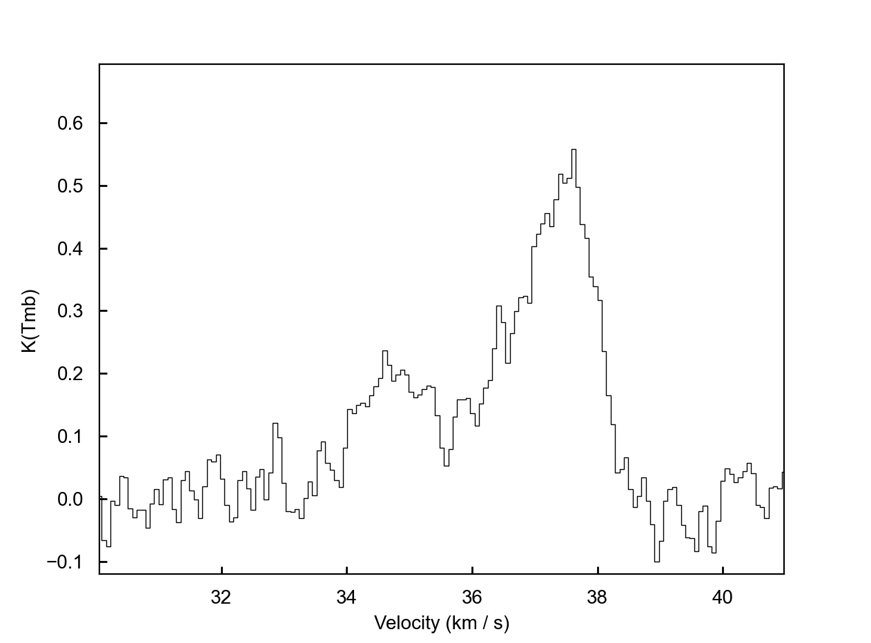
An important note on this data set is that N2H+ (1-0) has hyperfine structure. For the purposes of this tutorial, we are going to fit only the isolated hyperfine component. Specific to this data set, this component is located between ~ 30-41 km/s.

Stage 0: preparation step¶

The first thing we are going to do is import scousepy using

from scousepy import scouse

Next, we want to tell scousepy where the data is and where to output the files associated with each stage

datadir='/path/to/the/data/'
outputdir='/path/to/output/information/'
filename='n2h+10_37'

Note how the filename is provided without the .fits extension. If outputdir is not provided scousepy will output everything to datadir by default.

Now we are going to create the configuration files

config_file=scouse.run_setup(filename, datadir, outputdir=outputdir)

This will produce a directory with the following structure

| filename
| ├── config_files
| │   ├── scousepy.config
| │   ├── coverage.config
| ├── stage_1
| ├── stage_2
| ├── stage_3
| └── stage_4

scousepy.config will have the following structure

[DEFAULT]

# location of the FITS data cube you would like to decompose
datadirectory = '/path/to/the/data/'

# name of the FITS data cube (without extension)
filename = 'n2h+10_37'

# output directory for data products
outputdirectory = '/path/to/output/information/'

# decomposition model (default=Gaussian)
fittype = 'gaussian'

# Number of CPUs used for parallel processing
njobs = 3

# print messages to the terminal [True/False]
verbose = True

# autosave output from individual steps [True/False]
autosave = True

[stage_1]

# save moment maps as FITS files [True/False]
write_moments = True

# generate a figure of the coverage map [True/False]
save_fig = True

[stage_2]

# outputs an ascii table of the fits [True/False]
write_ascii = True

[stage_3]

# Tolerance values for the fitting. See Henshaw et al. 2016a
tol = [2.0,3.0,1.0,2.5,2.5,0.5]

Each of these parameters can be edited directly before running the subsequent stages. In particular, though scousepy performs much quicker in parallelised mode (njobs), debugging may be easier in serial.

coverage.config will have the following structure

[DEFAULT]

# number of refinement steps
nrefine = 1

# mask data below this value
mask_below = 0.0

# optional input filepath to a fits file containing a mask used to define the coverage
mask_coverage = None

# data x range in pixels
x_range = [None, None]

# data y range in pixels
y_range = [None, None]

# data velocity range in cube units
vel_range = [None, None]

# width of the spectral averaging areas
wsaa = [3]

# fractional limit below which SAAs are rejected
fillfactor = [0.5]

# sample size for randomly selecting SAAs
samplesize = 0

# method used to define the coverage [regular/random]
covmethod = 'regular'

# method setting spacing of SAAs [nyquist/regular]
spacing = 'nyquist'

# method defining spectral complexity
speccomplexity = 'momdiff'

# total number of SAAs
totalsaas = None

# total number of spectra within the coverage
totalspec = None

Again, each of these keywords can be edited manually before running stage 1. The GUI application of stage 1 can be bypassed using the keyword interactive=False.

Stage 1: defining the coverage - interactive¶

By default, scousepy will launch an interactive GUI in order to define the coverage…

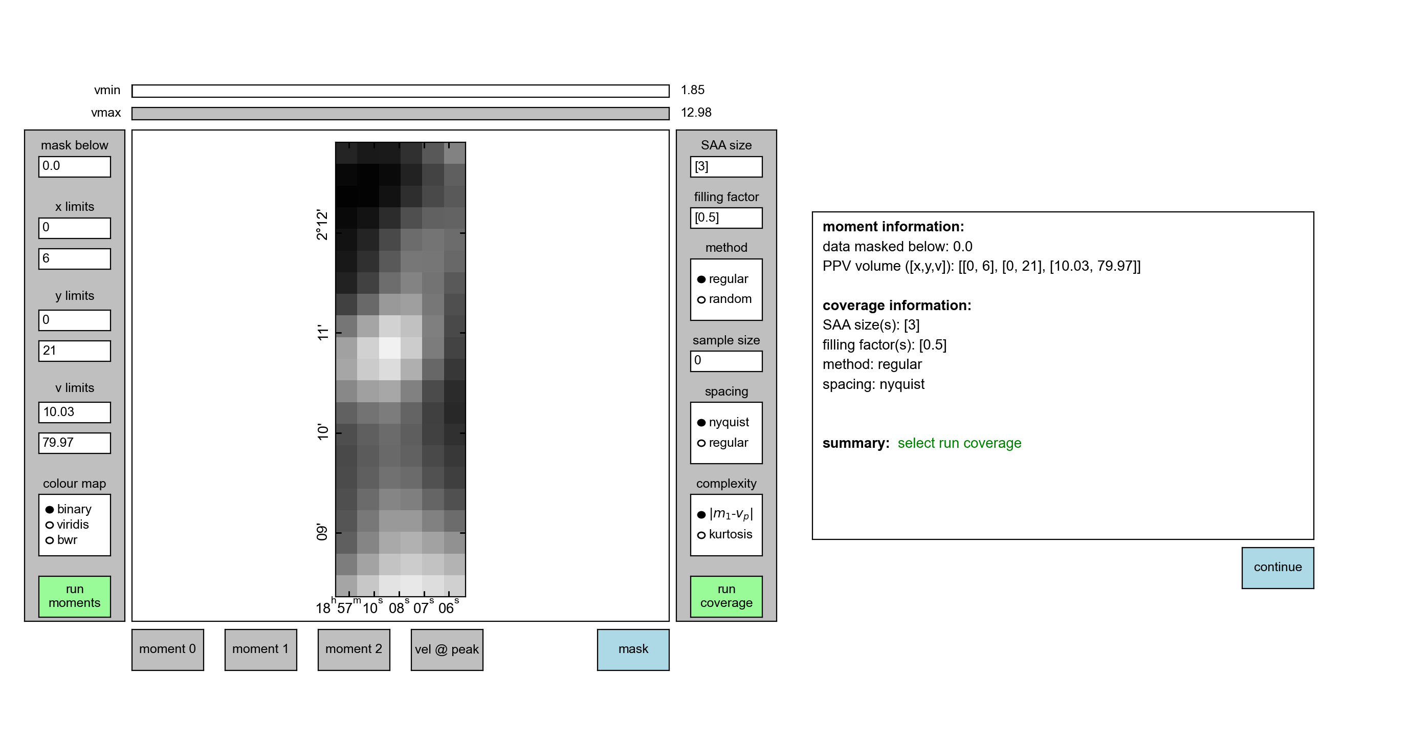
The keywords included in coverage.config are updated by interacting with the GUI. For this particular data set we are fitting N2H+ (1-0), so the first thing we want to do is truncate the velocity range over which we are going to perform the fitting such that we only focus our attention on the isolated hyperfine component. We can do this by adjusting the v limits boxes and clicking run moments. The v limits are given in absolute units whereas the x limits and y limits should be given in pixel units. This will result in the following

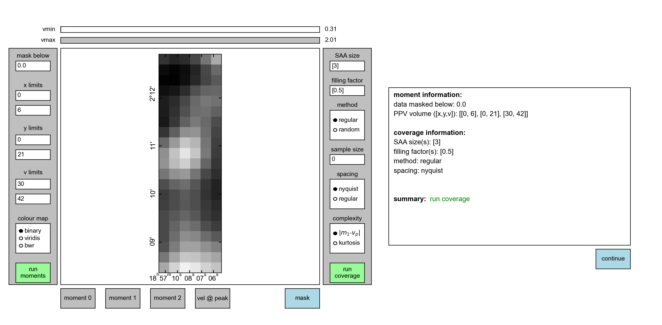
Note how although the image itself doesn’t change much, the intensity does. This can be inferred from the sliders at the top of the GUI.

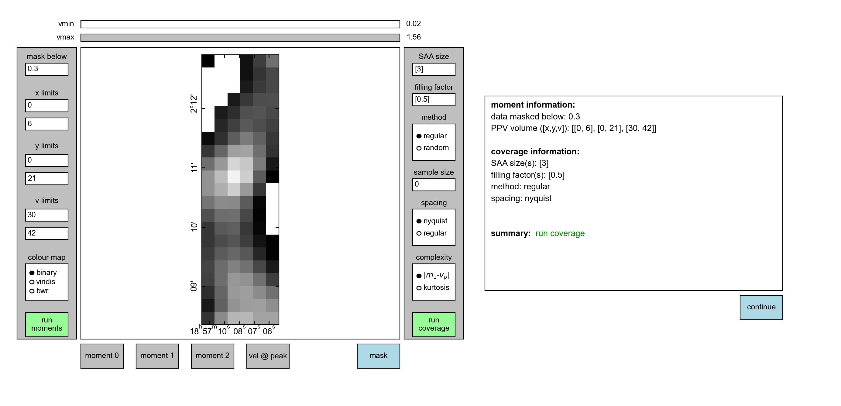
We can also apply a mask such that we only fit a portion of the data. Here I have used a mask of 0.3 (again in absolute units, in this case K), remembering to click run moments again,

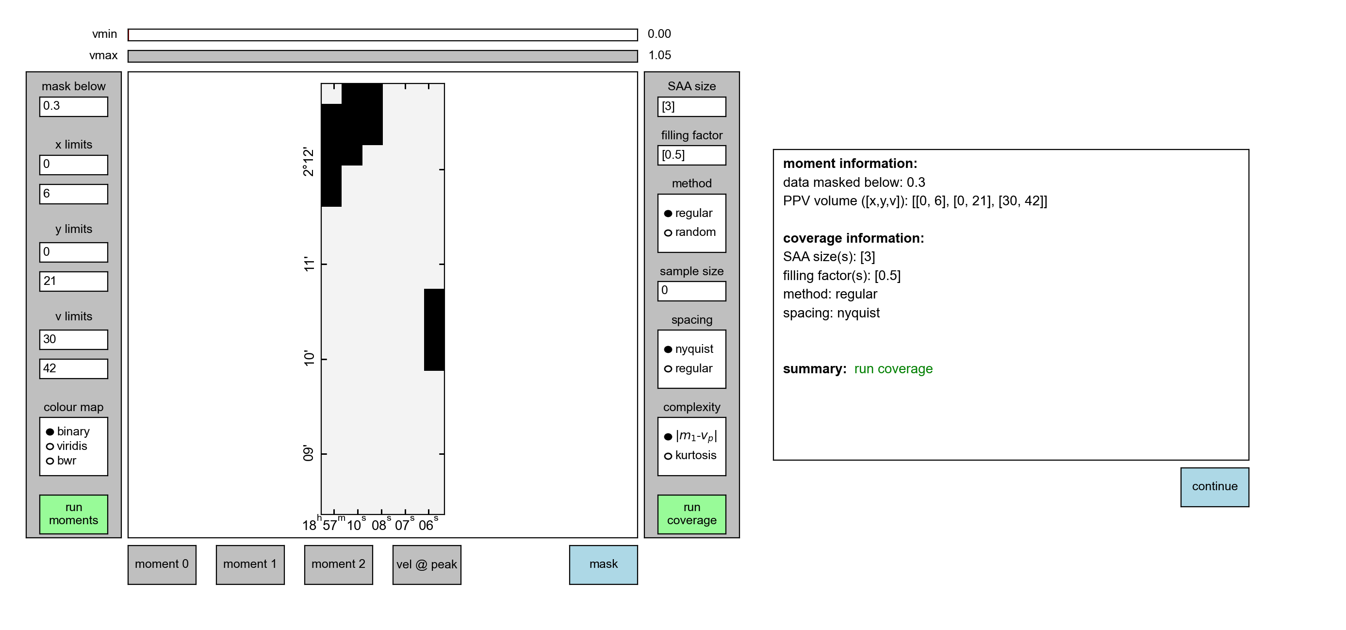
We can inspect the mask itself by clicking on the mask button at the bottom

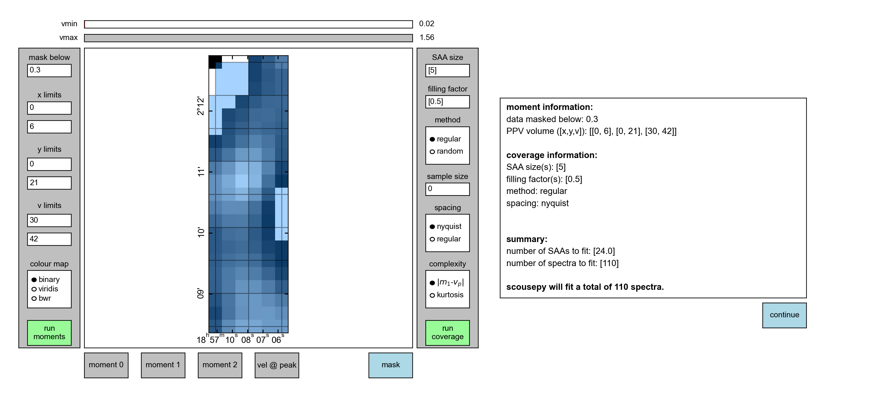
Next up we want to run the coverage. For this we first want to set the SAA size. Here I have set the SAA size=5. I have also retained the default settings for the other options, most importantly the filling factor=0.5. Clicking on run coverage will produce the coverage map.

The remaining settings are best ignored for now, but relate to various pieces of code that are still in development. The coverage will be displayed on the image and the box to the right will now display some basic statistics. Most importantly it indicates how many SAAs are to be fit and how many spectra are included within those SAAs (and will therefore be fit during stage 3).

Done correctly, you should see something like this

Hitting continue will process the coverage and extract the spatially averaged spectra from each of the spectral averaging areas

Stage 1: defining the coverage - non-interactive¶

Note that the coverage.config file can be edited directly to perform the computation of the coverage in a non-interactive way. Personally, I have found this helpful when fitting multiple cubes. In a separate code, I might extract information on the velocity limits using simple moment analysis. I can then update the configuration file using something like the following

from scousepy.configmaker import ConfigMaker

# create a dictionary for updating the scouse config file
mydicts={'datadirectory': datadir,
        'filename': cubename,
        'outputdirectory': outputdir,
        'njobs': njobs,
        'tol': tol}

# create a dictionary for updating the coverage config file
mydictc={'mask_coverage':maskfile,
        'mask_below':snr*rms,
        'vel_range':[velmin.value, velmax.value],
        'wsaa': [wsaa],
        'fillfactor': [fillfactor]}

ConfigMaker(pathto_scousepyconfig, configtype='init', dict=mydicts)
ConfigMaker(pathto_coverageconfig, configtype='coverage', dict=mydictc)

Note how you can use a pre-defined mask here as opposed to using the moment based method used in the interactive version of stage 1. To run stage 1 in this way use

s = scouse.stage_1(config=config_file, interactive=False)

Stage 2: fitting the spectral averaging areas¶

Stage 2 is where we will perform our semi-automated fitting. Running the following command will initiate a GUI that will allow us to fit the SAA spectra

s = scouse.stage_2(config=config_file)

Where the GUI will look like this

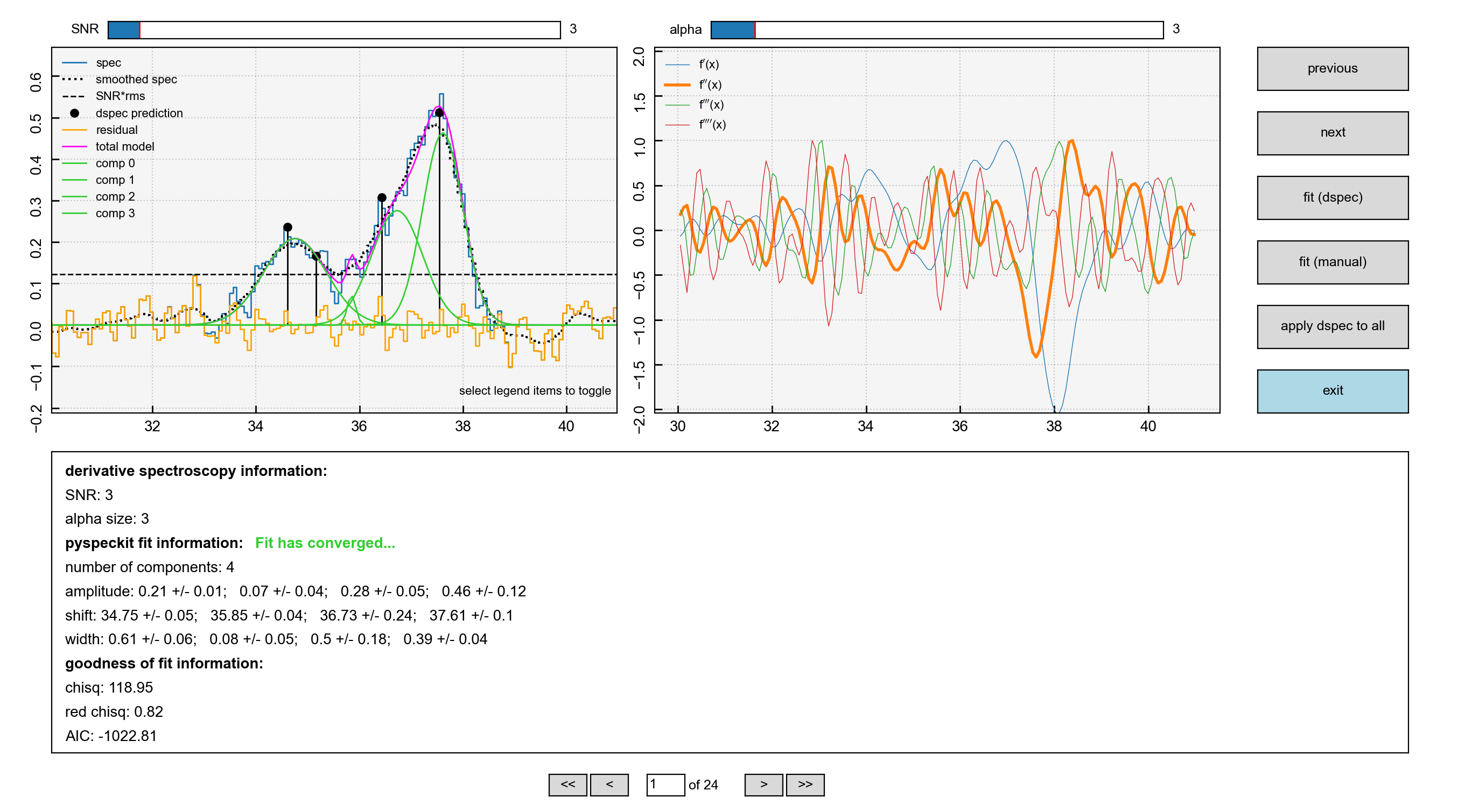
The GUI is divided into three main regions (not including the navigation buttons at the right and bottom of the screen). The top-left displays:

The spectrum to be fit (blue solid histogram)
A spectrum that has been smoothed with a Gaussian Kernel of width=alpha (black dotted curve)
The initial guesses indicated the location and amplitude of peaks derived from derivative spectroscopy (black lollipops)
Fitted components (green curves)
The total model indicating the sum of the individual components (magenta curve)
The residuals (orange histogram) defined as the spectrum-model

Each of these items can be toggled on/off by clicking on the markers in the legend.

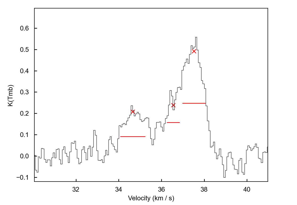
The top-right displays the first (blue), second (orange), third (green), and fourth (red) order derivatives of the smoothed spectrum displayed in the left-hand plot. The profiles of these curves are used to identify peaks in the data.

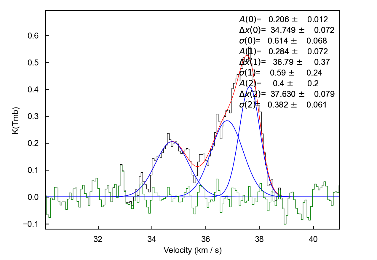
The bottom panel displays the fit information extracted from pyspeckit. First it tells us that the fit has converged. It tells us the number of fitted components and their Gaussian characteristics (amplitude, shift=centroid, and width) and uncertainties. It also shows us some goodness of fit statistics.

The fitting is controlled via the alpha and SNR parameters. As an example increasing the alpha value, which has the effect of smoothing the spectrum even more would result in a fewer number of components, as is illustrated here

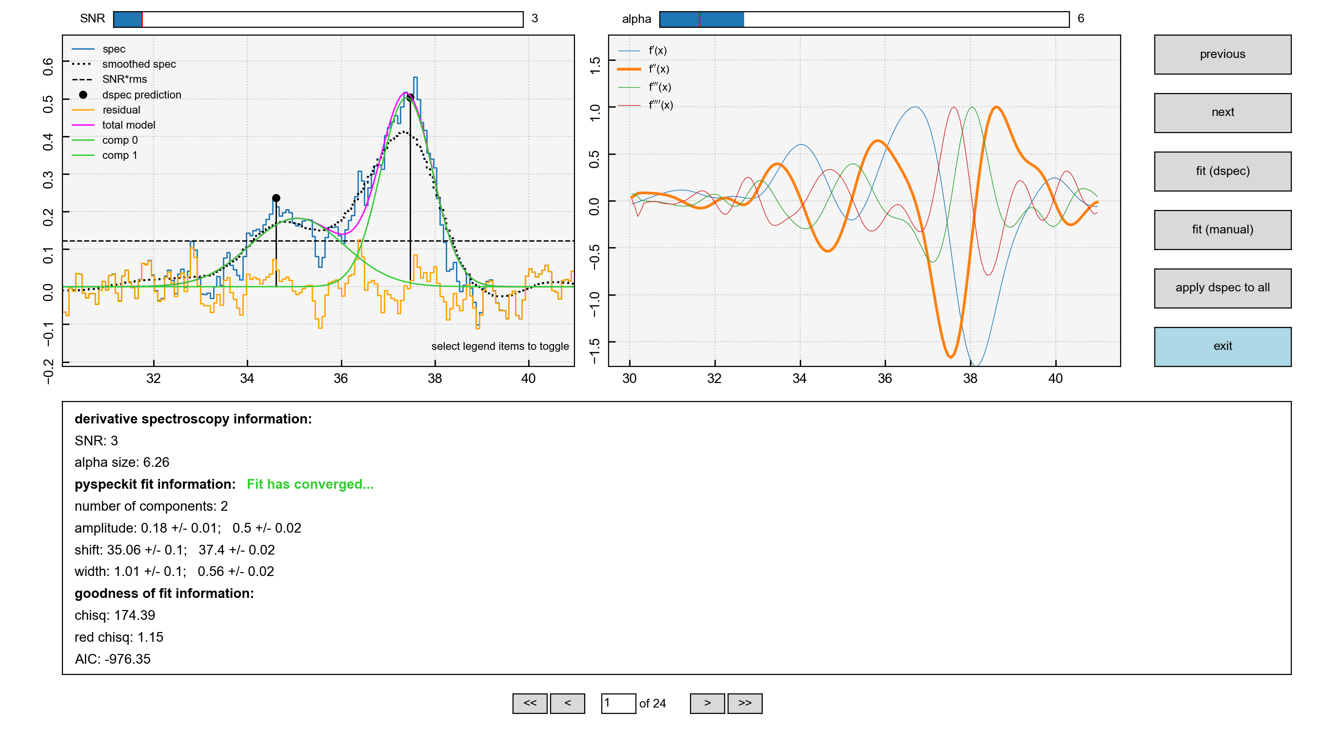
Note the difference in the right-hand panel, where now there are two prominent dips in the second derivative (orange) indicating the location of peaks.

If you are unable to find a suitable fit by adjusting the SNR and alpha sliders, the other option is to enter the manual fitter which can be found in the navigation bar on the right. This will open up pyspeckit’s manual fitter and should look like this

Interactive fitting can be performed using several commands. To indicate the components that you would like to fit, you select each component twice: once somewhere close to the peak emission and another click to indicate (roughly) the full-width at half-maximum. In my experience with this, you don’t need to be particularly accurate, pyspeckit does an excellent job of picking up the components you have selected. Selection can be made either using the keyboard (m) or mouse. Once selected this will look something like this…

If you are happy with your fit, hitting d will lock it in. The resulting fit will be plotted and some useful information will be printed out to the terminal.

Hitting enter will close the interactive window and the fit in scousepy’s stage 2 GUI will update.

You can then navigate to the next spectra either by using the navigation bar on the right (previous, next) or the buttons at the bottom. Note that if at any time you exit the fitter, and re-run the script, scousepy will pick up where it left off.

Finally, when checking the results of the automated fitting in stage 3 and 4, it may become clear that some tweaks are needed to the fitting. Using the keyword refit will allow you to re-enter the fitter

s = scouse.stage_2(config=config_file, refit=True)

You can then navigate to problematic spectra using the input field at the bottom of the GUI.

Stage 3: automated fitting¶

Stage 3 represents the automated decomposition stage. scousepy will take you best-fitting solutions from stage 2 and pass these to the individual spectra located within each SAA. The fitting process is controlled by a number of tolerance levels which are passed to scousepy via the tol keyword in scousepy.config.

The tolerance levels are descibed more completely in Henshaw et al. 2016. However, in short, the tolerance levels correspond to the following

The allowed change in the number of components between the fit of an individual spectrum and its parent SAA.
The S/N ratio each component must satisfy.
The minimum width of each component given as a multiple of the channel spacing.
This controls how similar a component must be to the closest matching component in the SAA fit in terms of velocity dispersion.
This controls how similar a component must be to the closest matching component in the SAA fit in terms of centroid velocity.
This governs the minimum separation between two components for them to be considered distinguishable (it is given as a multiple of the width of the narrowest component).

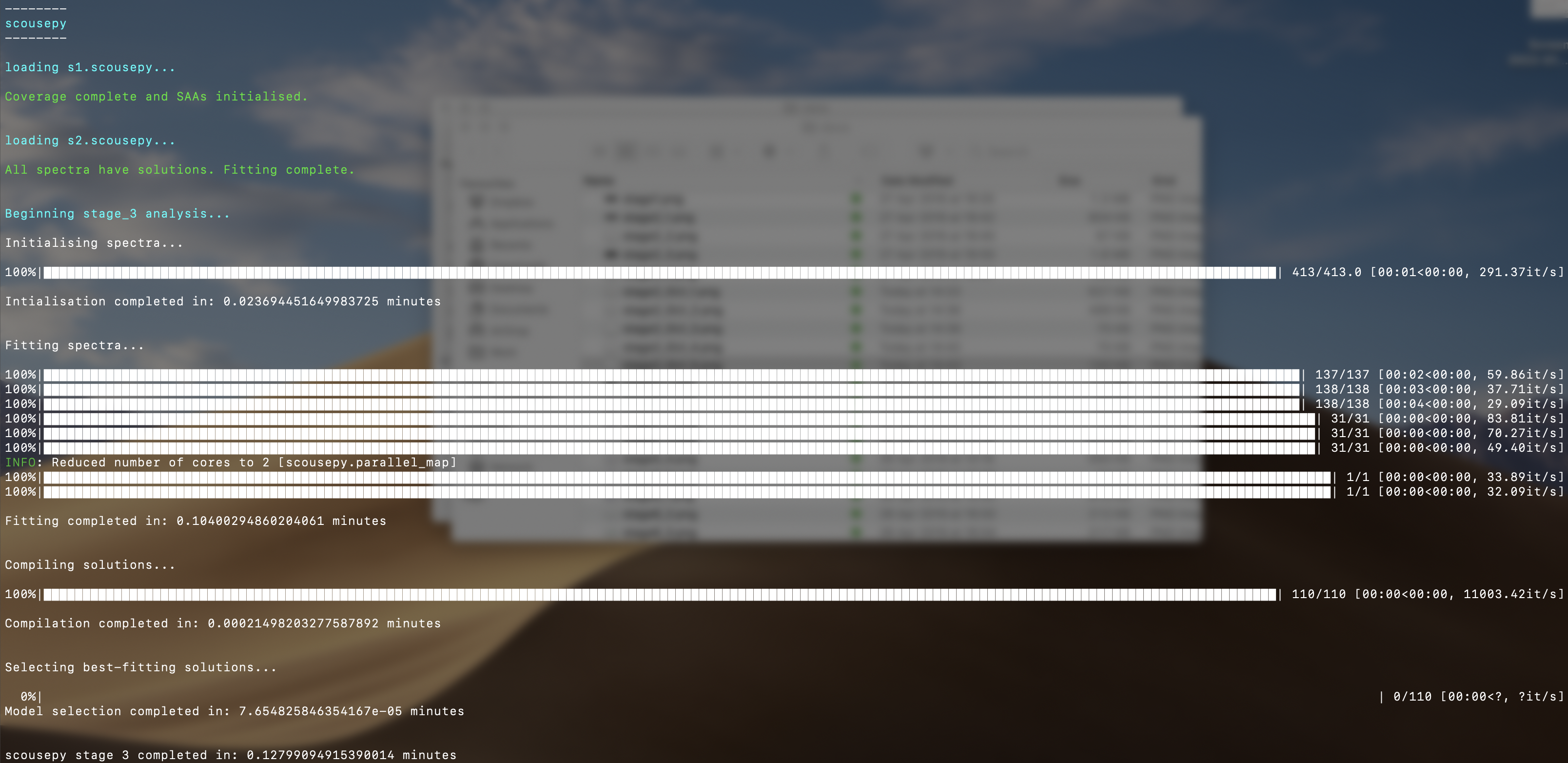
Stage 3 is run using the following command

s = scouse.stage_3(config=config_file)

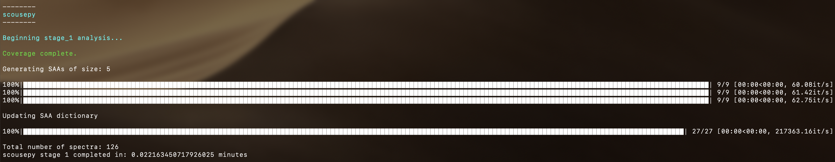
with the progress report output to terminal

The Nyquist sampling of the SAAs means that a given spectrum may have multiple solutions. scousepy identifies the best-fitting solution via the Akaike Information Criterion (AIC). The AIC is a measure of relative fitting quality which is used for fitting evaluation and model selection. The decision is in favour of the model with the lowest AIC. The AIC is given

\[\mathrm{AIC}=2(k-L)\]

in which \(k\) is the number of free parameters, and \(L\) is the log likelihood function of the model evaluated at the maximum likelihood estimate (i. e., the parameters for which L is maximized). More generally, scousepy computes the AIC assuming that the observations are Gaussian distributed such that

\[\mathrm{AIC}=n\,\mathrm{ln}\bigg(\frac{SSR}{n}\bigg)+2k\]

in which \(SSR\) is the sum of the squared residuals and \(n\) is the sample size. In the event that the sample size is not large enough \(n<40\), a correction is applied

\[\mathrm{AIC}=n\,\mathrm{ln}\bigg(\frac{SSR}{n}\bigg)+2k+\frac{2k(k+1)}{n-k-1}.\]

The computation is handled via astropy.

To select the best-fitting solution, scousepy uses the following rule of thumb from Burnham and Anderson 2002, pg. 70:

\[\Delta \mathrm{AIC}_{i}=\mathrm{AIC}_{i}-\mathrm{AIC}_{min}\]

\[\Delta \mathrm{AIC}_{i}<2\;\mathrm{substantial\;support\;for\;model}\;i\]

\[4<\Delta \mathrm{AIC}_{i}<7\;\mathrm{considerably\;less\;support\;for\;model}\;i\]

\[\Delta \mathrm{AIC}_{i}>10\;\mathrm{essentially\;no\;support\;for\;model}\;i\]

where \(\mathrm{AIC}_{min}\) is the minimum \(\mathrm{AIC}\) value out of the models compared.

Something to consider is the njobs keyword. Various stages of scousepy have been parallelised. The parallelisation works on a divide and conquer approach, whereby the total number of spectra to be fit are divided into batches and each batch sent to a different cpu. I would highly recommend using njobs>1 for large (>10000 spectra) data sets or for data sets with large numbers of components.

Stage 4: quality control¶

Stage 4 represents the quality control phase. Here we are able to inspect the decomposition. Stage 4 is run using the following command

s = scouse.stage_4(config=config_file)

This command will launch a GUI with which we can inspect the best-fitting solutions determined during stage 3. The GUI will look like the following

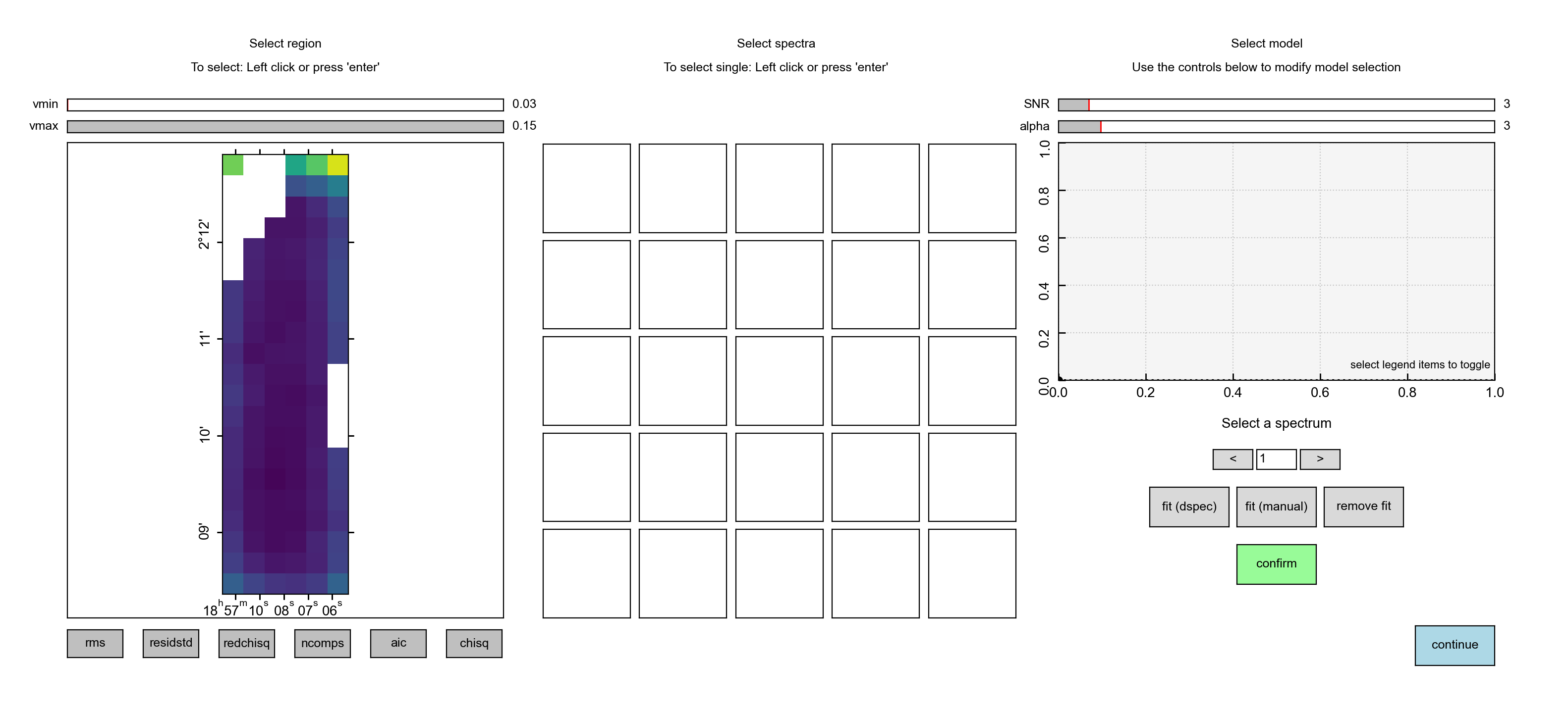
The GUI is divided into three main areas. The left panel displays a series of diagnostic plots that can be used to identify problem areas. The diagnostic plots include

rms noise.
standard deviation of the residual spectrum at each pixel
reduced \(\chi^{2}\)
number of fitted components
AIC - the Akaike Information Criterion
\(\chi^{2}\)

Selecting a pixel in the diagnostic map will display the spectrum and its best-fitting solution at that location (as well as its surrounding neighbours) in the central panel like so

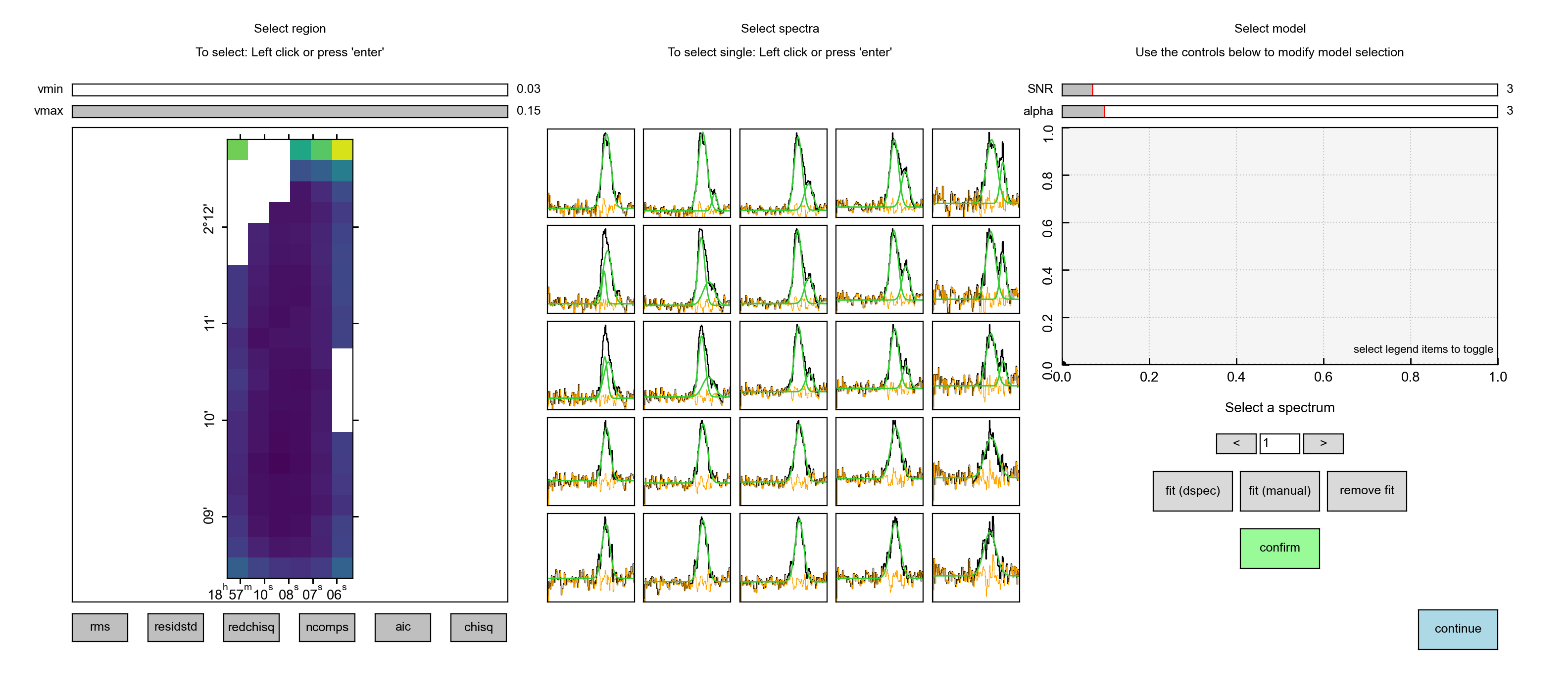
The user can then select one of the highlighted spectra for closer inspection. By clicking on one of the spectra in the central panel, it will appear in the right-hand panel. Underneath the spectrum will include some additional information on the decomposition. In the example below, we can see that there are two models available. The model selected (and displayed) by scousepy is a two component model.

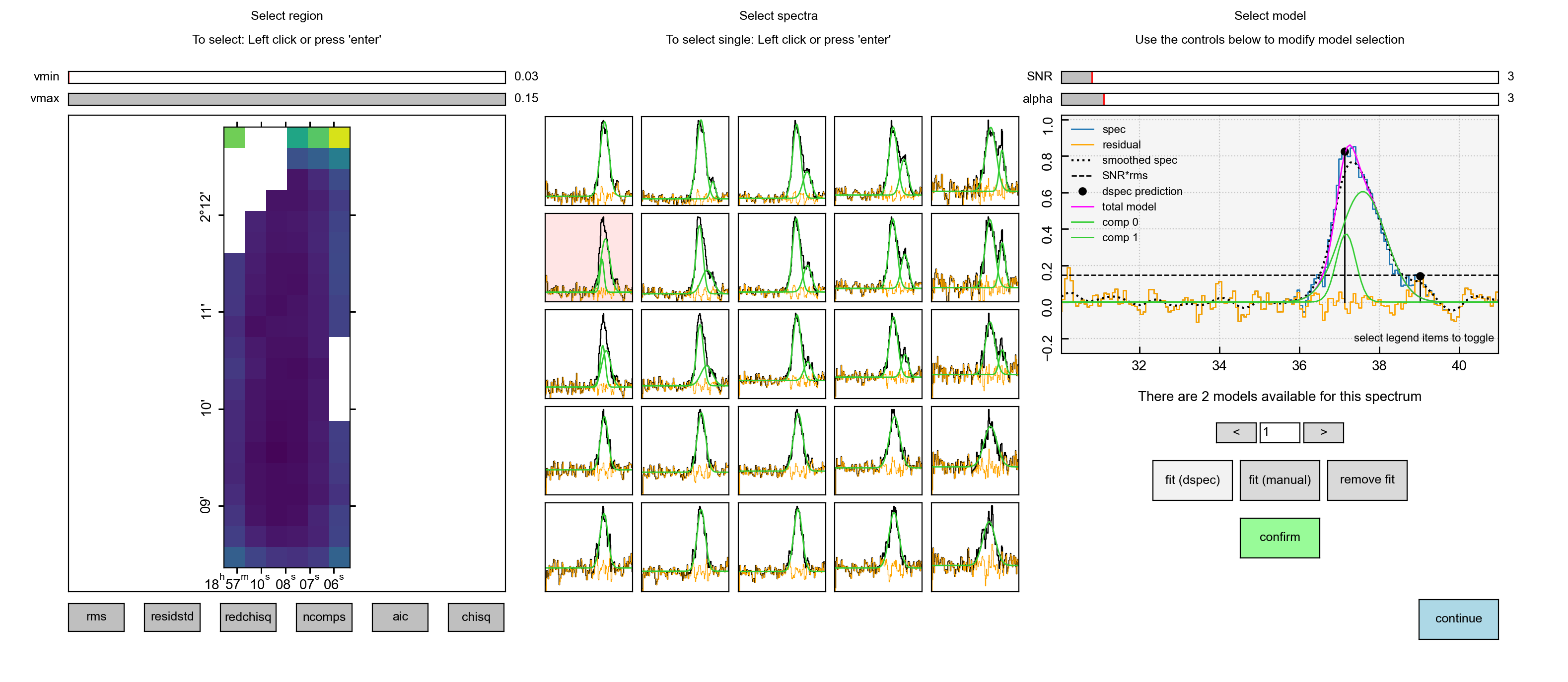
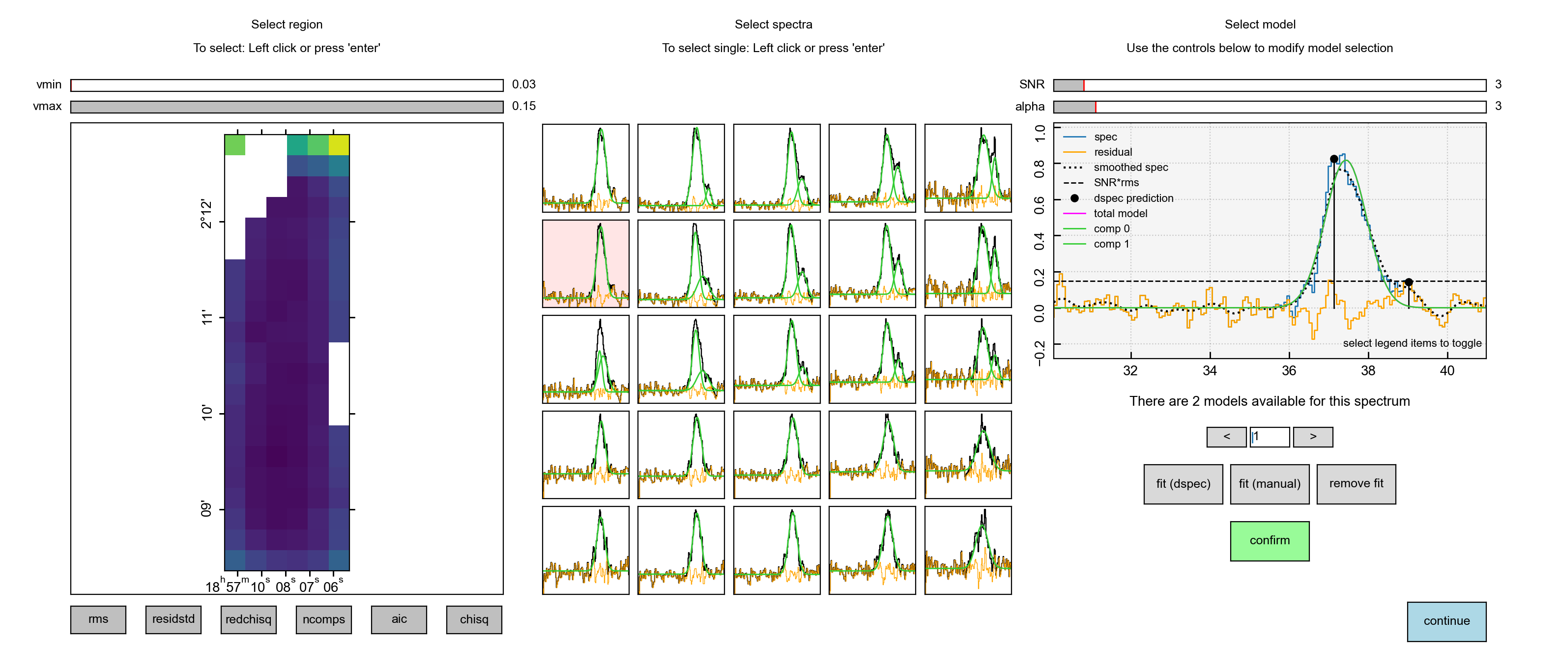
However, the user has the option to edit this. Pressing on the right arrow will display the next available solution, in this case, a single component fit. If the user would like to use this solution instead, they can click confirm. Note how this automatically updates the spectrum model in the central panel.

Alternatively, the user can manually fit the spectrum, either using derivative spectroscopy fit (dspec) or manually using fit (manual), which will launch pyspeckit’s manual fitter. Again, to lock the change in, the user must hit confirm before selecting another spectrum.

The user can end the process by hitting continue. If at any stage the user would like to re-enter this quality control step, they can do so by using the keyword bitesize

s = scouse.stage_4(config=config_file, bitesize=True)

Note that the user can also bypass this step entirely by using the keyword nocheck

s = scouse.stage_4(config=config_file, nocheck=True)

A complete example¶

To run all the steps in sequence your code might look something like this

# import scousepy
from scousepy import scouse

# create pointers to input, output, data
datadir='/path/to/the/data/'
outputdir='/path/to/output/information/'
filename='n2h+10_37'

# run scousepy
config_file=scouse.run_setup(filename, datadirectory, outputdir=outputdir)
s = scouse.stage_1(config=config_file, interactive=True)
s = scouse.stage_2(config=config_file)
s = scouse.stage_3(config=config_file)
s = scouse.stage_4(config=config_file, bitesize=True)

Navigation