A brief introduction to scousepy
Spectral decomposition with scousepy is broken up into a sequence of distinct
stages. Each stage is summarised below. More information on executing each of
these steps can be found in the tutorials.
Stage 0: preparation step
The preparation step involves the creation of configuration files that scousepy
will use to run the fitting. The first is scousepy.config. This contains the
top-level information for fitting including information on the directory structure,
the number of cpus for parallelised fitting, and optional keywords. The second is
coverage.config. This contains all relevant information for the definition of
the coverage (stage 1).
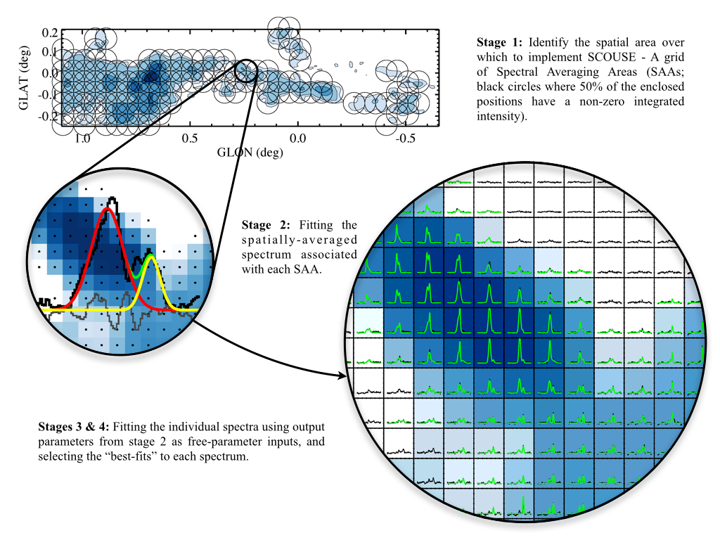
Stage 1: defining the coverage
Here scousepy identifies the spatial area over which to fit the data. There
are two different ways this can be achieved: 1) via an interactive GUI; 2) via
the configuration file ``coverage.config’’.
Both methods generate a grid of spectral averaging areas (SAAs). In the
interactive mode, scousepy will generate moment maps based on user defined
variables that are supplied as keywords within a matplotlib GUI. These
optional keywords include a mask threshold as well as ranges in the x,
y, and velocity axes. In the non-interactive mode, the keywords are supplied
via ``coverage.config’’. The user can also port a ready made mask for the
coverage definition via the mask_coverage keyword, which should be a path
to a FITS file which will act as the mask.
In defining the coverage the user must supply the size of the SAAs, which is
provided via wsaa (corresponding to the width, in pixels, of the SAA). The
user can also provide a filling factor via fillfactor. This keyword will
allow scousepy to reject all SAAs, where the fractional number of significant
pixels contained within a given SAA does not satisfy this constraint. Extra
refinement of the SAAs (i.e. for complex regions) can be controlled using the
keyword refine_grid. By default, the SAAs are Nyquist sampled. This means
that any given spectrum may have multiple solutions.
Stage 2: fitting the spectral averaging areas
User-interactive fitting of the spatially averaged spectra output from stage 1. Running stage 2 will launch a GUI for interactive fitting of the spectra extracted from the SAAs.
scousepy uses a technique called derivative spectroscopy to provide initial
guesses for the decomposition of the SAA spectra. Derivative spectroscopy
identifies peaks in the data by computing the derivatives of the spectrum
(shown in the top-left panel of the GUI). The method is controlled by two
parameters that can be adjusted using the sliders at the top of the GUI,
SNR and alpha. The former is the signal-to-noise requirement for all identified
peaks, and the latter controls the kernel size for smoothing of the spectrum.
Smoothing is required to avoid noise amplification in the derivative spectra.
The fit from derivative spectroscopy can be overruled by initiating the interactive fitter from pyspeckit.
The user can navigate through the spectra using the buttons at the bottom of the
GUI. The user may also choose to apply derivative spectroscopy to all of the
spectra using the default (or current) values of SNR and alpha.
Stage 3: automated fitting
Non user-interactive fitting of the individual spectra contained within all SAAs.
The user is required to input several tolerance levels to scousepy. Please
refer to Henshaw et al. 2016
for more details on each of these. These are supplied via the scousepy.config
file.
The Nyquist sampling of the SAAs means that a given spectrum may have multiple
solutions. scousepy identifies the best-fitting solution via the Akaike
Information Criterion (AIC). The AIC is a measure of relative fitting quality
which is used for fitting evaluation and model selection. The decision is in
favour of the model with the lowest AIC. The AIC is given
in which \(k\) is the number of free parameters, and \(L\) is the log
likelihood function of the model evaluated at the maximum likelihood estimate
(i. e., the parameters for which L is maximized). More generally, scousepy
computes the AIC assuming that the observations are Gaussian distributed such
that
in which \(SSR\) is the sum of the squared residuals and \(n\) is the sample size. In the event that the sample size is not large enough \(n<40\), a correction is applied
The computation is handled via astropy.
To select the best-fitting solution, scousepy uses the following rule of
thumb from Burnham and Anderson 2002, pg. 70:
where \(\mathrm{AIC}_{min}\) is the minimum \(\mathrm{AIC}\) value out of the models compared.
Stage 4: quality control
Quality control of the best-fitting solutions derived in stage 3. Running stage 4 will launch a GUI displaying various diagnostic plots of the goodness-of-fit statistics output by the decomposition. Clicking on this image will display a grid of spectra in the central panel for closer inspection. Clicking on one of those spectra will plot the selected spectrum in the right-hand panel. At this point the user has the option to select an alternative model solution (if available) or re-enter the fitting procedure, either using derivative spectroscopy or via the manual fitting procedure implemented in pyspeckit.